
With tracking, we can expect to see a plot of the following for ADC, a small pedestal with a tail on the right hand side that represents the physics. This data will get picked up in the following way, for an event, the track from the TPC will be matched with a tower and with a preshower. However, if the mapping is WRONG, we will in fact be reading data from a neighbouring preshower. When we then plot the ADC for the preshower we will not "see" the physics as the neighboring channel had the real hit, we will just see preshower pedestal events in the selected tower channel
The 2D plots that were made before began an investigation into this effect by plotting, with no TPC information, hits above pedestal. This was made over all combinations of tower and preshower in an event. We can now take this further and investigate the case with tracking for the ADC spectra.
Previously, a majority of the mapping problems are found at fixed intervals of +20 or +40 channels. Adams files are unique to this analysis because they not only record hits made on a channel where the Preshower is equal to the Tower, with tracking from the TPC, but they also record hits made on the 8 surrounding towers (Array 1-8 in the picture).
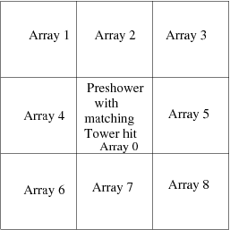
This information was recorded for clustering analysis but can be used as a preliminary investigation into the mapping as well. If the top/middle and bottom/middle array (index 2 and 7) increase by +/- one channel, they will lay along the same sub-module. This would put the left/middle and right/middle arrays (index 4 and 6 in diagram) on the neighbouring sub-modules, which are separated by +/-20 channels.
We can therefore directly check mappings that are off by +/- 20 channels simply by comparing the spectra from channel "0", with array "4" and "8".
Note: This will not pick up mapping problems that were off by different amounts, such as the common +/- 40, or by "backward" wired channels where the increasing Preshower ID saw a decreasing Tower ID correlation in the 2d plots, but these can be investigated with modifications to this method
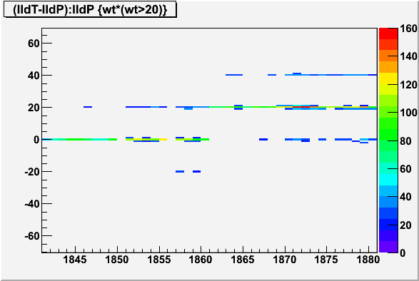
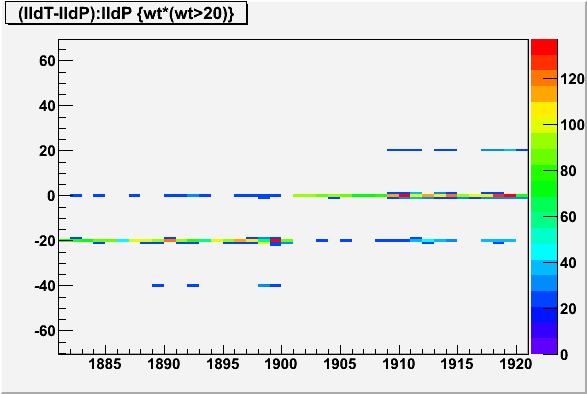
From the 2D plots made previously, for the channels between 1861 and 1900. Looking at the 2D plot the channels are seen to be +20 from 1861 to 1880 and then -20 from 1881 to 1900. This is the pattern we would expect from a bad mapping. This is because the preshower from twenty channels over is being hit. The pattern of +20 for 1861-1880 then -20 from 1881-1900 further enforces the "bad mapping" hypothesis, as the preshower channel shows the channel where the real hit was, followed, as we move further along, by the 'reflection' where the real hit shows the correct preshower channel.
http://www4.rcf.bnl.gov/~rfc/mapping_v3/mapping_scan/1-2400_1841.png
http://www4.rcf.bnl.gov/~rfc/mapping_v3/mapping_scan/1-2400_1881.png
This pattern is also seen in the spectra when we use Adams files. In the following plot, we look at the spectra for a good channel, 1240
The top plot is the ADC of the preshower, the bottom left and the bottom right are the ADC from -20 and +20 channels, these data come from the clusting information recorded in the file, see array index "4" and "6" in the previous picture. Each "fill" will have the same amount of events. The conditon means that the tracking=preshower=tower for this plot and the mapping was correct as there is the "physics" tail. The histogram has a higher RMS due to this physics tail. For the preshowers from the neighbouring modules (minus and plus 20), all that was recorded were pedestal hits, and no physics, as expected, so these peaks are narrow and with smaller RMS

Now look at a plot with a bad mapping, channel 1861 has been interchanged, twenty channels, with 1881. For the readout preshower channels, the top plot is just pedestal in both examples. The mapping means that the channel just reads pedestal hits. If we look at neighbouring towers, where the events really map to, we see high RMS and events with tails, first in 1861 (Minus) and then the reflection in 1881 (Plus)

For all the plots from this analysis please follow these links
All the plots from 1-2400 are here! All the plots from 2401-4800 are here!By scanning the plots we can look for bad mappings using the following algorithm:
Using this method, the following list of mapping problems was generated, Will Jacobs has produced a list of bad channels and we can see here that the method accurately reproduced most of Will's list for channels that were off by +/-20. These have a "w" on the left hand side.
Some channels were not re-produced, such as 266,286,287,633,634,638,644,653,654. On looking that the plots for these cases, it seems that there is a strong signal in the preshower and the mapping worked here.
List from the comparison method
The method found mostly all the 20 channel mappings from Will's list. The examples from this list that it skipped did not seem to be the pattern expected from +/-20 channel shifts in the ADC spectra
The change in the ADC spectra's RMS, with tracking, seems to be a way to identify bad mappings. The "physics" will increase the tail and change the RMS. Comparing the RMS of spectra to +/- "x channels" seems to identify problems with mapping that are swapped by "x" channels
We can also use this method to read +/-40 and reversed wired channels. It could then supplement the 2D plot method and identify bad mappings in a faster and more rigorous way.
Another advantage is that we only use the preshower(tower) spectra, this should only identify problems with the preshower(tower) mapping.
We can try these methods on the Cu-Cu preshower data and see how well the mapping worked there